Showing posts with label cpk. Show all posts

Friday, September 11, 2009

Capability Analysis in JMP

I received a note asking how to do a capability analysis in JMP 8. Actually nothing much have changed in how to do it. There are additional features which are really helpful but the basic steps on computing Cp, Cpk, Pp, and Ppk are basically shared by versions JMP 5, JMP 6, JMP 7, and JMP 8. Here are the detailed steps. I will be using JMP 8's sample data 'Semiconductor Capability.jmp'.

Capability Analysis in JMP

Method1
Step1: Data Requirements
Data should be in one column and data type set as continuous.
Step2: Go to Univariate Platform
Create a histogram of your measurement data as shown below.
Step3: Click on the second hot button
It is the red triangle as shown below. On the drop down menu, select 'Capability Analysis'
Step4: Specification Limits
On the resulting dialog box, fill up the necessary information regarding the specification limits and target values. In this case they are 104.41295,118.15322, and 131.89349. For Pp and Ppk, check on the tick box 'Long Term Sigma'. For Cp and Cpk, select either on the tick box 'Moving Range...' and specify the range span, or on the tick box 'Short Term Sigma...'. Note that whichever you choose JMP would use the terms Cp and Cpk in its output. It would specify in the title box of the output though the Sigma your analysis is referring to.
Step5: Capability Analysis Output
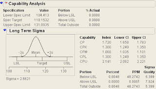
After pressing 'OK', JMP will give you this output.

Method2:
Step1: Data Requirements
Same as above
Step2: Set up the column that contains your data
Right click on the column header to see the following menu. Select 'Column Info'.
Step3: Column Properties
On the drop down menu 'Column Properties', select 'Spec Limits'.
Step4:Specification Limits
Fill up the necessary information regarding the specification limits and target values. In this case they are 104.41295,118.15322, and 131.89349, and then click 'OK'. Notice on the left side of your data table, and asterisk (*) sign is placed beside the column name where you just set up the specification limits.
Step5: Go to Univariate Platform
Create a histogram of your measurement data as shown below. Capability Analysis using Long Term Sigma is included by default.

Additional Features:
One of the reasons why I favor JMP over Minitab is its animated graphics. In JMP 8, Capability Analysis includes a feature called 'Capability Animation. To use this, click on the hot button as shown below.
The output window is like the one shown below.You can change the sigma to see its impact on the capability measures. For a JMP script like this where you can change the mean as well, refer to this entry or this entry.

Thursday, August 6, 2009

Cp vs Cpk: Illustrating the Impact of Mean Shift and Sigma Changes

This is a script I developed to help me in explaining the concepts of Cp/Pp and Cpk/Ppk whenever I am conducting Six Sigma trainings. This is one of the reasons I appreciate JMP's JSL. It allows me to customize demostrations for my trainees that visually aid them in grasping Six Sigma concepts.
You may freely use. I would be grateful if you would give the credit to me and refer to this blog.

Reynald Francisco
http://statisticalprocesscontrols.blogspot.com/


The JMP JSL Script


dlg = Dialog(
V List(V List("Cpk Parameters","",
Line Up(2,
"Mean", mu = Edit Number(0),
"Standard Deviation", sigma = Edit Number(1)
),"","",
"Define Specifications","",
Line Up( 2,
"USL ",USL = Edit Number(2)
),Line Up( 2,
"LSL ",LSL = Edit Number(-2)
)
),
H List( Button("OK"), Button("Cancel") )
));


If( dlg["Button"] == -1, Throw( "User cancelled" ) );
Remove From( dlg ); Eval List( dlg );


rsqrt2pi = 1/sqrt(2*pi());

New Window("Cpk Demostration",

Graph Box(
FrameSize(500,500),
XScale(mu-8*sigma,mu+8*sigma),
yScale(0,1.40*rsqrt2pi/sigma),
Double Buffer,
Pencolor("blue"),
pensize(1),
text size(12),
TextColor("black"),
YFunction(Normal Density((x-mu)/sigma)/sigma, x); /*Y-scale is Normalized to Z-scores*/
YFunction(Normal Density((x-mu)/sigma)/sigma, x,fill(20),max(LSL)); /*Fill low*/
YFunction(Normal Density((x-mu)/sigma)/sigma, x,fill(20),min(USL)); /*Fill high*/
Handle(mu,rsqrt2pi/sigma,mu=x;sigma=rsqrt2pi/y);
Pencolor("red"),
pensize(1),
text size(10),
TextColor("black"),
XFunction(LSL, y);
Handle(LSL,0.45*rsqrt2pi/sigma,LSL=x);
XFunction(USL, y);
Handle(USL,0.55*rsqrt2pi/sigma,USL=x);
text({mu,0.85*rsqrt2pi/sigma},"mu ",mu," sigma ",sigma);
textcolor("red");
text({LSL,0.45*rsqrt2pi/sigma},"LSL= ",LSL);
text({USL,0.55*rsqrt2pi/sigma},"USL= ",USL);
Pencolor("blue"),
pensize(1),
text size(11),
TextColor("blue"),
Cpu=(USL-mu)/(3*sigma);
Zu=(USL-mu)/sigma;
Zl=(LSL-mu)/sigma;
yield=normal distribution(Zu)- normal distribution(Zl);
Cpl=(mu-LSL)/(3*sigma);
Cpk=min(Cpu,Cpl);
text({mu,1.15*rsqrt2pi/sigma},"Cpk= ",Cpk);
text({mu,1.35*rsqrt2pi/sigma},"Cpu= ",Cpu);
text({mu,1.25*rsqrt2pi/sigma},"Cpl= ",Cpl);
text({mu,1.05*rsqrt2pi/sigma},"Estimated Yield= ",yield);
) /* Close Graph Box parenthesis*/
); /* Close New Window parenthesis*/

Thursday, July 30, 2009

Process Capability Measures Cp and Cpk: A JMP JSL Demostration

I am often asked about the diffence between Cp and Cpk. Usually it is followed up by a question on why there is a need for two measures. I then answer that while Cpk is the real capability, Cp reflects the potential capability that can still be achieved just by centering your process. This is a difficult concept to grasp if just verbally described, so I usually illustrate this using a graphical demostration.
This JMP script demostrates the differences between the two Process Capability Measures Cp and Cpk.


The JMP JSL Script


dlg = Dialog(
V List(
V List(
"Cp Parameters",
"",
Line Up( 2,
/*"Mean", mu = Edit Number(0),*/
"Standard Deviation", sigma = Edit Number( 1 )
),
"",
"",
"Define Specifications",
"",
Line Up( 2, "USL ", upspecs = Edit Number( 2 ) ),
Line Up( 2, "LSL ", lowspecs = Edit Number( -2 ) )
),
H List( Button( "OK" ), Button( "Cancel" ) )
)
);


If( dlg["Button"] == -1,
Throw( "User cancelled" )
);
Remove From( dlg );
Eval List( dlg );


/*ADDED line for Cp only*/
LSL = lowspecs;
USL = upspecs;
mu = lowspecs + (upspecs - lowspecs) / 2;
mid = (upspecs - lowspecs);
/*END of added line*/


rsqrt2pi = 1 / Sqrt( 2 * Pi() );

New Window( "Process Capability Demostration",
V List Box(
H List Box(
Panel Box( "Cpk Window",
T1=Text Box ("Move the Handle in the curve to change the value of the Mean"),
g1 = Graph Box(
FrameSize( 425, 400 ),
X Scale( mu - 8 * sigma, mu + 8 * sigma ),
Y Scale( 0, 1.40 * rsqrt2pi / sigma ),
Double Buffer,
Pen Color( "blue" ),
Pen Size( 1 ),
Text Size( 12 ),
Text Color( "black" ),
Y Function( Normal Density( (x - mu) / sigma ) / sigma, x ); /*Y-scale is Normalized to Z-scores*/
Y Function(
Normal Density( (x - mu) / sigma ) / sigma,
x,
fill( 20 ),
Max( LSL )
); /*Fill low*/
Y Function(
Normal Density( (x - mu) / sigma ) / sigma,
x,
fill( 20 ),
Min( USL )
); /*Fill high*/
Pen Color( "red" );,
Pen Size( 1 ),
Text Size( 10 ),
Text Color( "black" ),
X Function( LSL, y );
Handle( mu, rsqrt2pi / sigma, mu = x;g2<<reshow; );
g2 << reshow;
Handle( LSL, 0.45 * rsqrt2pi / sigma, LSL = x );
g2 << reshow;
Handle( USL, 0.45 * rsqrt2pi / sigma, USL = x );
X Function( USL, y );
delta = mu - LSL;
Text( {mu, 0.85 * rsqrt2pi / sigma}, "mu ", mu, " sigma ", sigma );
Text Color( "red" );
Text( {LSL, 0.45 * rsqrt2pi / sigma}, "LSL= ", LSL );
Text( {USL, 0.55 * rsqrt2pi / sigma}, "USL= ", USL );
Pen Color( "blue" );,
Pen Size( 1 ),
Text Size( 11 ),
Text Color( "blue" ),
Cp = (USL - LSL) / (6 * sigma);
Cpu = (USL - mu) / (3 * sigma);
Zu = (USL - mu) / sigma;
Zl = (LSL - mu) / sigma;
yield = Normal Distribution( Zu ) - Normal Distribution( Zl );
Cpl = (mu - LSL) / (3 * sigma);
Cpk = Min( Cpu, Cpl );
Text( {mu, 1.25 * rsqrt2pi / sigma}, "Cpk= ", Cpk );
Text( {mu, 1.15 * rsqrt2pi / sigma}, "Cp= ", Cp );
Text( {mu, 1.05 * rsqrt2pi / sigma}, "Estimated Yield= ", yield );
) /* Close Graph Box parenthesis*/
),
Panel Box( "Cp Window",
T2=Text Box ("Move the Handle in the curve to change the value of the Sigma");,
g2 = Graph Box(
FrameSize( 425, 400 ),
X Scale( mu - 8 * sigma, mu + 8 * sigma ),
Y Scale( 0, 1.40 * rsqrt2pi / sigma ),
Double Buffer,
Handle( mu, rsqrt2pi / sigma, sigma = rsqrt2pi / y; g1<<reshow; );
delta = mu - LSL;
USL2 = mu + delta;
Pen Color( "red" );,
Pen Size( 1 ),
Text Size( 10 ),
Text Color( "black" ),
X Function( LSL, y );
X Function( USL2, y );
Text( {mu, 0.85 * rsqrt2pi / sigma}, "mu ", mu, " sigma ", sigma );
Text Color( "red" );
Text( {LSL, 0.45 * rsqrt2pi / sigma}, "LSL= ", LSL );
Text( {USL2, 0.55 * rsqrt2pi / sigma}, "USL= ", USL2 );
Pen Color( "blue" );,
Pen Size( 1 ),
Text Size( 11 ),
Text Color( "blue" ),
Cpu = (USL2 - mu) / (3 * sigma);
Zu = (USL2 - mu) / sigma;
Zl = (LSL - mu) / sigma;
yield2 = Normal Distribution( Zu ) - Normal Distribution( Zl );
Cpl = (mu - LSL) / (3 * sigma);
Cp2 = (USL2 - LSL) / (6 * sigma);
Text( {mu, 1.15 * rsqrt2pi / sigma}, "Cp= ", Cp2 );
Text( {mu, 1.05 * rsqrt2pi / sigma}, "Estimated Yield= ", yield2 );
Pen Color( "blue" );,
Pen Size( 1 ),
Text Size( 12 ),
Text Color( "black" ),
Y Function( Normal Density( (x - mu) / sigma ) / sigma, x ); /*Y-scale is Normalized to Z-scores*/
Y Function(
Normal Density( (x - mu) / sigma ) / sigma,
x,
fill( 20 ),
Max( LSL )
); /*Fill low*/
Y Function(
Normal Density( (x - mu) / sigma ) / sigma,
x,
fill( 20 ),
Min( USL2 )
); /*Fill high*/
)
)
)
)/*END Of BORDER BOX*/
); /* Close New Window parenthesis*/

T1<<Text Color("BLUE");
T2<<Text Color("BLUE");

Sunday, July 26, 2009

Sigma Level as a Measure of Process Capabiltity (Reposted from www.SixSigmaPractice.multiply.com

There are many available measures of Process Capability.
In fact anything that relates process variation to specification
limits,and measures how often the process meets these specifications can be considered as a measure of Process Capability.
Process Capability can be measured either by Percent Yield, Percent Defect, Cp, Pp, Cpk, Ppk, or Sigma Level. This JSL script uses JMP's graphical capability to demostrate how the standard Normal Curve defines the relationships between the Sigma Level, percent Yield, and percent defect.
 
Note: You may use freely but the author will appreciate it the author will be given credit, and this webpage will be sited.
Reynald Francisco
http://www.sixsigmapractice.multiply.com/


The JMP JSL Script

When the JMP script is run, an initial dialog box would prompt the user the input initial values as shown below.
Input Dialog Box:


The output image is a graph as shown below:


The JMP JSL Script is shown below::

dlg = Dialog(
V List(
V List(
"ENTER THE FOLLOWING INFORMATION:",
"",
V List(
"Input Option",
V List(
TestType = Radio
Buttons( "YIELD RATE", "DEFECT RATE", "SIGMA LEVEL" ),
Line Up( 2, "Input
Value ", x = Edit Number( 0.5 ) )
)
),
"",
"Note: Input Yield
Rate and Defect Rate in decimal format."
),
H List( Button( "OK" ),
Button( "Cancel" ) )
)
);

If( dlg["Button"] == -1,
Throw(
"User cancelled" )
);
Remove From( dlg );
Eval List( dlg );

If(
TestType != 3 & x >= 1,
Caption( "Input Yield Rate
and Defect Rate in decimal format. Right click to close message." );
Throw(
"User cancelled" );,
TestType != 3 & x <= 0,
Caption( "Input
value is not valid. Right click to close message." );
Throw( "User
cancelled" );,
TestType == 3 & x < 0,
Caption( "Input value is
not valid. Right click to close message." );
Throw( "User cancelled" );
);

mu = 0;
sigma = 1;
rsqrt2pi = 1 / Sqrt( 2 * Pi() );

If(
TestType == 3, SigmaLevel = x,
TestType == 1, SigmaLevel =
Normal Quantile( x ),
TestType == 2, SigmaLevel = Normal Quantile( 1 - x )
);

New Window( "Sigma Level Demostration",
Graph Box(
FrameSize( 900, 500 ),
X Scale( -10, 10 ),
Y Scale( 0, 0.5 ),
Double Buffer,
Pen Color( "blue" ),
Pen Size( 1 ),
Text Size( 12
),
Text Color( "black" ),
Y Function( Normal Density( (x - mu) / sigma )
/ sigma, x ); /*Y-scale is Normalized to Z-scores*/
If( TestType == 2,
Y
Function( Normal Density( (x - mu) / sigma ) / sigma, x, fill( 1 ), Min(
SigmaLevel ) ),
Y Function( Normal Density( (x - mu) / sigma ) / sigma, x,
fill( 1 ), Max( SigmaLevel ) )
);
Pen Color( "red" );,
Pen Size( 1
),
Text Size( 10 ),
Text Color( "black" ),
X Function( SigmaLevel, y
);
Handle( SigmaLevel, 0.45 * rsqrt2pi / sigma, SigmaLevel = x );
Text
Color( "black" );
Text( {SigmaLevel, 0.45 * rsqrt2pi / sigma}, "<--Move
this point" );
Text Color( "red" );
Text( {SigmaLevel, 0.55 * rsqrt2pi /
sigma}, "Sigma Level= ", SigmaLevel );
Pen Color( "blue" );,
Pen Size( 1
),
Text Size( 11 ),
Text Color( "blue" ),
Z = (SigmaLevel - mu) /
sigma;
Yield = Normal Distribution( Z );
Defect = (1 - Yield);
Text(
{mu, 1.15 * rsqrt2pi / sigma}, "YIELD= ", yield * 100, "%" );
Text( {mu,
1.05 * rsqrt2pi / sigma}, "DEFECT= ", defect * 100, "%" );
) /* Close Graph
Box parenthesis*/
); /* Close New Window parenthesis*/


Custom Search